Participants in “Recomposing the Humanities,” September 2015. Pictured from left to right: Barbara Herrnstein Smith, Rita Felski, Bruno Latour, Nigel Thrift, Michael Witmore, Dipesh Chakrabarti, and Stephen Muecke.
Abstract: Talk about the humanities today tends to focus on their perceived decline at the expense of other, more technical modes of inquiry. The big S “sciences” of nature, we are told, are winning out against the more reflexive modes of humanistic inquiry that encompass the study of literature, history, philosophy, and the arts. This decline narrative suggests we live in a divided kingdom of disciplines, one composed of two provinces, each governed by its own set of laws. Enter Bruno Latour, who, like an impertinent Kent confronting an aging King Lear, looks at the division of the kingdom and declares it misguided, even disastrous. Latour’s narrative of the modern bifurcation of knowledge sits in provocative parallel with the narrative of humanities-in-decline: what humanists are trying to save (that is, reflexive inquiry directed at artifacts) was never a distinct form of knowledge. It is a province without borders, one that may be impossible to defend. We are now in the midst of a further plot turn with the arrival of digital methods in the humanities, methods that seem to have strayed into our province from the sciences. As this new player weaves in and out of the plots I have just described, some interesting questions start to emerge. Does the use of digital methods in the humanities represent an incursion across battle lines that demands countermeasures, a defense of humanistic inquiry from the reductive methods of the natural or social sciences? Will humanists lose something precious by hybridizing with a strain of knowledge that sits on the far side of the modern divide? What is this precious thing that might be lost, and whose is it to lose?
Rembrandt, The Denial of St. Peter (1660), Rijksmuseum
In the “Fortunata” chapter of his landmark study, Mimesis: The Representation of Reality, Eric Auerbach contrasts two representations of reality, one found in the New Testament Gospels, the other in texts by Homer and a few other classical writers. As with much of Auerbach’s writing, the sweep of his generalizations is broad. Long excerpts are chosen from representative texts. Contrasts and arguments are made as these excerpts are glossed and related to a broader field of texts. Often Auerbach only gestures toward the larger pattern: readers of Mimesis must then generate their own (hopefully congruent) understanding of what the example represents.
So many have praised Auerbach’s powers of observation and close reading. At the very least, his status as a “domain expert” makes his judgments worth paying attention to in a computational context. In this post, I want to see how a machine would parse the difference between the two types of texts Auerbach analyzes, stacking the iterative model against the perceptions of a master critic. This is a variation on the experiments I have performed with Jonathan Hope, where we take a critical judgment (i.e., someone’s division of Shakespeare’s corpus of plays into genres) and then attempt to reconstruct, at the level of linguistic features, the perception which underlies that judgment. We ask, Can we describe what this person is seeing or reacting to in another way?
Now, Auerbach never fully states what makes his texts different from one another, which makes this task harder. Readers must infer both the larger field of texts that exemplify the difference Auerbach alludes to, and the difference itself as adumbrated by that larger field. Sharon Marcus is writing an important piece on this allusive play between scales — between reference to an extended excerpt and reference to a much larger literary field. Because so much goes unstated in this game of stand-ins and implied contrasts, the prospect of re-describing Auerbach’s difference in other terms seems particularly daunting. The added difficulty makes for a more interesting experiment.
Getting at Auerbach’s Distinction by Counting Linguistic Features
I want to offer a few caveats before outlining what we can learn from a computational comparison of the kinds of works Auerbach refers to in his study. For any of what follows to be relevant or interesting, you must take for granted that the individual books of the Odyssey and the New Testament Gospels (as they exist in translation from Project Gutenberg) represent adequately the texts Auerbach was thinking about in the “Fortunata” chapter. You must grant, too, that the linguistic features identified by Docuscope are useful in elucidating some kind of underlying judgments, even when it is used on texts in translation. (More on the latter and very important point below.) You must further accept that Docuscope, here version 3.91, has all the flaws of a humanly curated tag set. (Docuscope annotates all texts tirelessly and consistently according to procedures defined by its creators.) Finally, you must already agree that Auerbach is a perceptive reader, a point I will discuss at greater length below.
I begin with a number of excerpts that I hope will give a feel for the contrast in question, if it is a single contrast. This is Auerbach writing in the English translation of Mimesis:
[on Petronius] As in Homer, a clear and equal light floods the persons and things with which he deals; like Homer, he has leisure enough to make his presentation explicit; what he says can have but one meaning, nothing is left mysteriously in the background, everything is expressed. (26-27)
[on the Acts of the Apostles and Paul’s Epistles] It goes without saying that the stylistic convention of antiquity fails here, for the reaction of the casually involved person can only be presented with the highest seriousness. The random fisherman or publican or rich youth, the random Samaritan or adulteress, come from their random everyday circumstances to be immediately confronted with the personality of Jesus; and the reaction of an individual in such a moment is necessarily a matter of profound seriousness, and very often tragic.” (44)
[on Gospel of Mark] Generally speaking, direct discourse is restricted in the antique historians to great continuous speeches…But here—in the scene of Peter’s denial—the dramatic tension of the moment when the actors stand face to face has been given a salience and immediacy compared with which the dialogue of antique tragedy appears highly stylized….I hope that this symptom, the use of direct discourse in living dialogue, suffices to characterize, for our purposes, the relation of the writings of the New Testament to classical rhetoric…” (46)
[on Tacitus] That he does not fall into the dry and unvisualized, is due not only to his genius but to the incomparably successful cultivation of the visual, of the sensory, throughout antiquity. (46)
[on the story of Peter’s denial] Here we have neither survey and rational disposition, nor artistic purpose. The visual and sensory as it appears here is no conscious imitation and hence is rarely completely realized. It appears because it is attached to the events which are to be related… (47, emphasis mine)
There is a lot to work with here, and the difference Auerbach is after is probably always going to be a matter of interpretation. The simple contrast seems to be that between the “equal light” that “floods persons and things” in Homer and the “living dialogue” of the Gospels. The classical presentation of reality is almost sculptural in the sense that every aspect of that reality is touched by the artistic designs of the writer. One chisel carves every surface. The rendering of reality in the Gospels, on the other hand, is partial and (changing metaphors here) shadowed. People of all kinds speak, encounter one another in “their random everyday circumstances,” and the immediacy of that encounter is what lends vividness to the story. The visual and sensory “appear…because [they are] attached to the events which are to be related.” Overt artistry is no longer required to dispose all the details in a single, frieze-like scene. Whatever is vivid becomes so, seemingly, as a consequence of what is said and done, and only as a consequence.
These are powerful perceptions: they strike many literary critics as accurately capturing something of the difference between the two kinds of writing. It is difficult to say whether our own recognition of these contrasts, speaking now as readers of Auerbach, is the result of any one example or formulation that he offers. It may be the case, as Sharon Marcus is arguing, that Auerbach’s method works by “scaling” between the finely wrought example (in long passages excerpted from the texts he reads) and the broad generalizations that are drawn from them. The fact that I had to quote so many passages from Auerbach suggests that the sources of his own perceptions are difficult to discern.
Can we now describe those sources by counting linguistic features in the texts Auerbach wants to contrast? What would a quantitative re-description of Auerbach’s claims look like? I attempted to answer these questions by tagging and then analyzing the Project Gutenberg texts of the Odyssey and the Gospels. I used the latest version of Docuscope that is currently being used by the Visualizing English Print team, a program that scans a corpus of texts and then tallies linguistic features according to a hand curated sets of words and phrases called “Language Action Types” (hereafter, “features”). Thanks to the Visualizing English Print project, I can share the raw materials of the analysis. Here you can download the full text of everything being compared. Each text can be viewed interactively according to the features (coded by color) that have been counted. When you open any of these files in a web browser, select a feature to explore by pressing on the feature names to the left. (This “lights up” the text with that feature’s color).
I encourage you to examine these texts as tagged by Docuscope for yourself. Like me, you will find many individual tagging decisions you disagree with. Because Docuscope assigns every word or phrase to one and only one feature (including the feature, “untagged”), it is doomed to imprecision and can be systematically off base. After some checking, however, I find that the things Docuscope counts happen often and consistently enough that the results are worth thinking about. (Hope and I found this to be the case in our Shakespeare Quarterly article on Shakespeare’s genres.) I always try to examine as many examples of a feature in context as I can before deciding that the feature is worth including in the analysis. Were I to develop this blog post into an article, I would spend considerably more time doing this. But the features included in the analysis here strike me as generally stable, and I have examined enough examples to feel that the errors are worth ignoring.
Findings
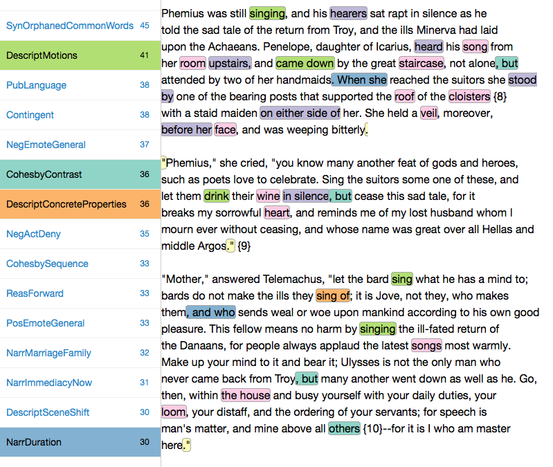
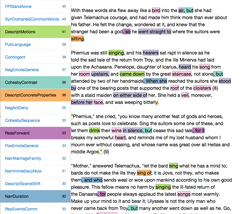
We can say with statistical confidence (p=<.001) that several of the features identified in this analysis are likely to occur in only one of the two types of writing. These and only these features are the ones I will discuss, starting with an example passage taken from the Odyssey. Names of highlighted features appear on the left hand side of the screen shot below, while words or phrases assigned to those features are highlighted in the text to the right. Again, items highlighted in the following examples appear significantly more often in the Odyssey than in the New Testament Gospels:
Odyssey, Book 1, Project Gutenberg Text (with discriminating features highlighted)
Book I is bustling with description of the sensuous world. Words in pink describe concrete objects (“wine,” “the house”, “loom”) while those in green describe things involving motion (verbs indicating an activity or change of state). Below are two further examples of such features:
Notice also the purple features above, which identify words involved in mediating spatial relationships. (I would quibble with “hearing” and “silence” as being spatial, per the long passage above, but in general I think this feature set is sound.) Finally, in yellow, we find a rather simple thing to tag: quotation marks at the beginning and end of a paragraph, indicating a long quotation.
Continuing on to a shorter set of examples, orange features in the passages below and above identify the sensible qualities of a thing described, while blue elements indicate words that extend narrative description (“. When she” “, and who”) or words that indicate durative intervals of time (“all night”). Again, these are words and phrases that are more prevalent in the Homeric text:
The items in cyan, particularly “But” and “, but” are interesting, since both continue a description by way of contrast. This translation of the Odyssey is full of such contrastive words, for example, “though”, “yet,” “however”, “others”, many of which are mediated by Greek particles in the original.
When quantitative analysis draws our attention to these features, we see that Auerbach’s distinction can indeed be tracked at this more granular level. Compared with the Gospels, the Odyssey uses significantly more words that describe physical and sensible objects of experience, contributing to what Auerbach calls the “successful cultivation of the visual.” For these texts to achieve the effects Auerbach describes, one might say that they can’t not use concrete nouns alongside adjectives that describe sensuous properties of things. Fair enough.
Perhaps more interesting, though, are those features below in blue (signifying progression, duration, addition) and cyan (contrastive particles), features that manage the flow of what gets presented in the diegesis. If the Odyssey can’t not use these words and phrases to achieve the effect Auerbach is describing, how do they contribute to the overall impression? Let’s look at another sample from the opening book of the Odyssey, now with a few more examples of these cyan and blue words:
Odyssey, Book 1, Project Gutenberg Text (with discriminating features highlighted)
While this is by no means the only interpretation of the role of the words highlighted here, I would suggest that phrases such as “when she”, “, and who”, or “, but” also create the even illumination of reality to which Auerbach alludes. We would have to look at many more examples to be sure, but these types of words allow the chisel to remain on the stone a little longer; they continue a description by in-folding contrasts or developments within a single narrative flow.
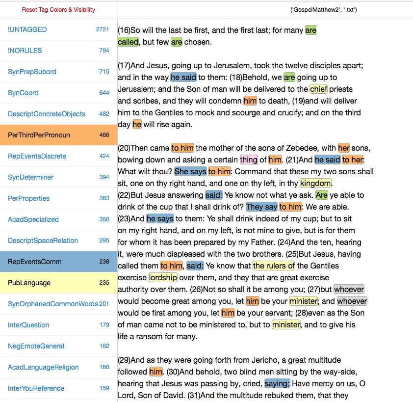
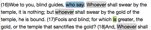
Let us now turn to the New Testament Gospels, which lack the above features but contain others to a degree that is statistically significant (i.e., we are confident that the generally higher measurements of these new features in the Gospels are not so by chance, and vice versa). I begin with a longer passage from Matthew 22, then a short passage from Peter’s denial of Jesus at Matthew 26:71. Please note that the colors employed below correspond to different features than they do in the passages above:
Matthew 22, Project Gutenberg Text (with discriminating features highlighted)
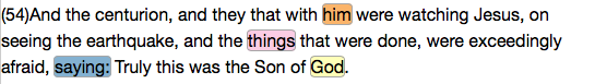
The dialogical nature of the Gospels is obvious here. Features in blue, indicating reports of communication events, are indispensable for representing dialogical exchange (“he says”, “said”, “She says”). Features in orange, which indicate uses of the third person pronoun, are also integral to the representation of dialogue; they indicate who is doing the saying. The features in yellow represent (imperfectly, I think) words that reference entities carrying communal authority, words such as “lordship,” “minister,” “chief,” “kingdom.” (Such words do not indicate that the speaker recognizes that authority.) Here again it is unsurprising that the Gospels, which contrast spiritual and secular forms of obligation, would be obliged to make repeated reference to such authoritative entities.
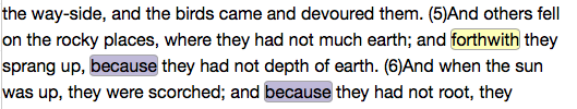
Things that happen less often may also play a role in differentiating these two kinds of texts. Consider now a group of features that, while present to a higher and statistically significant degree in the Gospels, are nevertheless relatively infrequent in comparison to the dialogical features immediately above. We are interested here in the words highlighted in purple, pink, gray and green:
Features in purple mark the process of “reason giving”; they identify moments when a reader or listener is directed to consider the cause of something, or to consider an action’s (spiritually prior) moral justification. In the quotation from Matthew 13, this form of backward looking justification takes the form of a parable (“because they had not depth…”). The English word “because” translates a number of ancient Greek words (διὰ, ὅτι); even a glance at the original raises important questions about how well this particular way of handling “reason giving” in English tracks the same practice in the original language. (Is there a qualitative parity here? If so, can that parity be tracked quantitatively?) In any event, the practice of letting a speaker — Jesus, but also others — reason aloud about causal or moral dependencies seems indispensable to the evangelical programme of the Gospels.
To this rhetoric of “reason giving” we can add another of proverbiality. The word “things” in pink (τὰ in the Greek) is used more frequently in the Gospels, as are words such as “whoever,” which appears here in gray (for Ὃς and ὃς). We see comparatively higher numbers of the present tense form of the verb “to be” in the Gospels as well, here highlighted in green (“is” for ἐστιν). (See the adage, “many are called, but few are chosen” in the longer Gospel passage from Matthew 22 excerpted above, translating Πολλοὶ γάρ εἰσιν κλητοὶὀλίγοι δὲ ἐκλεκτοί.)
These features introduce a certain strategic indefiniteness to the speech situation: attention is focused on things that are true from the standpoint of time immemorial or prophecy. (“Things” that just “are” true, “whatever” the case, “whoever” may be involved.). These features move the narrative into something like an “evangelical present” where moral reasoning and prophecy replace description of sensuous reality. In place of concrete detail, we get proverbial generalization. One further effect of this rhetoric of proverbiality is that the searchlight of narrative interest is momentarily dimmed, at least as a source illuminating an immediate physical reality.
What Made Auerbach “Right,” And Why Can We Still See It?
What have we learned from this exercise? Answering the most basic question, we can say that, after analyzing the frequency of a limited set of verbal features occurring in these two types of text (features tracked by Docuscope 3.91), we find that some of those features distribute unevenly across the corpus, and do so in a way that tracks the two types of texts Auerbach discusses. We have arrived, then, at a statistically valid description of what makes these two types of writing different, one that maps intelligibly onto the conceptual distinctions Auerbach makes in his own, mostly allusive analysis. If the test was to see if we can re-describe Auerbach’s insights by other means, Auerbach passes the test.
But is it really Auerbach who passes? I think Auerbach was already “right” regardless of what the statistics say. He is right because generations of critics recognize his distinction. What we were testing, then, was not whether Auerbach was “right,” but whether a distinction offered by this domain expert could be re-described by other means, at the level of iterated linguistic features. The distinction Auerbach offered in Mimesis passes the re-description test, and so we say, “Yes, that can be done.” Indeed, the largest sources of variance in this corpus — features with the highest covariance — seem to align independently with, and explicitly elaborate, the mimetic strategies Auerbach describes. If we have hit upon something here, it is not a new discovery about the texts themselves. Rather, we have found an alternate description of the things Auerbach may be reacting to. The real object of study here is the reaction of a reader.
Why insist that it is a reader’s reactions and not the texts themselves that we are describing? Because we cannot somehow deposit the sum total of the experience Auerbach brings to his reading in the “container” that is a text. Even if we are making exhaustive lists of words or features in texts, the complexity we are interested in is the complexity of literary judgment. This should not be surprising. We wouldn’t need a thing called literary criticism if what we said about the things we read exhausted or fully described that experience. There’s an unstatable fullness to our experience when we read. The enterprise of criticism is the ongoing search for ever more explicit descriptions of this fullness. Critics make gains in explicitness by introducing distinctions and examples. In this case, quantitative analysis extends the basic enterprise, introducing another searchlight that provides its own, partial illumination.
This exercise also suggests that a mimetic strategy discernible in one language survives translation into another. Auerbach presents an interesting case for thinking about such survival, since he wrote Mimesis while in exile in Istanbul, without immediate access to all of the sources he wants to analyze. What if Auerbach was thinking about the Greek texts of these works while writing the “Fortunata” chapter? How could it be, then, that at least some of what he was noticing in the Greek carries over into English via translation, living to be counted another day? Readers of Mimesis who do not know ancient Greek still see what Auerbach is talking about, and this must be because the difference between classical and New Testament mimesis depends on words or features that can’t be omitted in a reasonably faithful translation. Now a bigger question comes into focus. What does it mean to say that both Auerbach and the quantitative analysis converge on something non-negotiable that distinguishes these the two types of writing? Does it make sense to call this something “structural”?
If you come from the humanities, you are taking a deep breath right about now. “Structure” is a concept that many have worked hard to put in the ground. Here is a context, however, in which that word may still be useful. Structure or structures, in the sense I want to use these words, refers to whatever is non-negotiable in translation and, therefore, available for description or contrast in both qualitative and quantitative terms. Now, there are trivial cases that we would want to reject from this definition of structure. If I say that the Gospels are different from the Odyssey because the word Jesus occurs more frequently in the former, I am talking about something that is essential but not structural. (You could create a great “predictor” of whether a text is a Gospel by looking for the word “Jesus,” but no one would congratulate you.)
If I say, pace Auerbach, that the Gospels are more dialogical than the Homeric texts, and so that English translations of the same must more frequently use phrases like “he said,” the difference starts to feel more inbuilt. You may become even more intrigued to find that other, less obvious features contribute to that difference which Auerbach hadn’t thought to describe (for example, the present tense forms of “to be” in the Gospels, or pronouns such as “whoever” or “whatever”). We could go further and ask, Would it really be possible to create an English translation of Homer or the Gospels that fundamentally avoids dialogical cues, or severs them from the other features observed here? Even if, like the translator of Perec’s La Disparition, we were extremely clever in finding a way to avoid certain features, the resulting translation would likely register the displacement in another form. (That difference would live to be counted another way.) To the extent that we have identified a set of necessary, indispensable, “can’t not occur” features for the mimetic practice under discussion, we should be able to count it in both the original language as well as a reasonably faithful translation.
I would conjecture that for any distinction to be made among literary texts, there must be a countable correlate in translation for the difference being proposed. No correlate, no critical difference — at least, if we are talking about a difference a reader could recognize. Whether what is distinguished through such differences is a “structure,” a metaphysical essence, or a historical convention is beside the point. The major insight here is that the common ground between traditional literary criticism and the iterative, computational analysis of texts is that both study “that which survives translation.” There is no better or more precise description of our shared object of study.
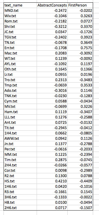
It’s hard to conceive of distance measured in anything other than a straight line. The biplot below, for example, shows the scores of Shakespeare’s plays on the two Docuscope LATs discussed in the previous post, FirstPerson and AbstractConcepts:
Plotting the items in two dimensions gives the viewer some general sense of the shape of the data. “There are more items here, less there.” But when it comes to thinking about distances between texts, we often measure straight across, favoring either a simple line linking two items or a line that links the perceived centers of groups.
The appeal of the line is strong, perhaps because it is one dimensional. And brutally so. We favor the simple line because want to see less, not more. Even if we are looking at a biplot, we can narrow distances to one dimension by drawing athwart the axes. The red lines linking points above — each the diagonal of a right triangle whose sides are parallel to our axes — will be straight and relatively easy to find. The line is simple, but its meaning is somewhat abstract because it spans two distinct kinds of distance at once.
Distances between items become slightly less abstract when things are represented in an ordered list. Scanning down the “text_name” column below, we know that items further down have less of the measured feature that those further up. There is a sequence here and, so, an order of sorts:
If we understand what is being measured, an ordered list can be quite suggestive. This one, for example, tells me that The Comedy of Errors has more FirstPerson tokens than The Tempest. But it also tells me, by virtue of the way it arranges the plays along a single axis, that the more FirstPerson Shakespeare uses in a play, the more likely it is that this play is a comedy. There are statistically precise ways of saying what “more” and “likely” mean in the previous sentence, but you don’t need those measures to appreciate the pattern.
What if I prefer the simplicity of an ordered list, but want nevertheless to work with distances measured in more than one dimension? To get what I want, I will have to find some meaningful way of associating the measurements on these two dimensions and, by virtue of that association, reducing them to a single measurement on a new (invented) variable. I want distances on a line, but I want to derive those distances from more than one type of measurement.
My next task, then, will be to quantify the joint participation of these two variables in patterns found across the corpus. Instead of looking at both of the received measurements (scores on FirstPerson and AbstractConcepts), I want to “project” the information from these two axes onto a new, single axis, extracting relevant information from both. This projection would be a reorientation of the data on a single new axis, a change accomplished by Principal Components Analysis or PCA.
To understand better how PCA works, let’s continue working with the two LATs plotted above. Recall from the previous post that these are the Docuscope scores we obtained from Ubiqu+ity and put into mean deviation form. A .csv file containing those scores can be found here. In what follows, we will be feeding those scores into an Excel spreadsheet and into the open source statistics package “R” using code repurposed from a post on PCA at Cross Validated by Antoni Parellada.
A Humanist Learns PCA: The How and Why
As Hope and I made greater use of unsupervised techniques such as PCA, I wanted a more concrete sense of how it worked. But to arrive at that sense, I had to learn things for which I had no visual intuition. Because I lack formal training in mathematics or statistics, I spent about two years (in all that spare time) learning the ins and outs of linear algebra, as well as some techniques from unsupervised learning. I did this with the help of a good textbook and a course on linear algebra at Kahn Academy.
Having learned to do PCA “by hand,” I have decided here to document that process for others wanting to try it for themselves. Over the course of this work, I came to a more intuitive understanding of the key move in PCA, which involves a change of basis via orthogonal projection of the data onto a new axis. I spent many months trying to understood what this means, and am now ready to try to explain or illustrate it to others.
My starting point was an excellent tutorial on PCA by Jonathon Shlens. Schlens shows why PCA is a good answer to a good question. If I believe that my measurements only incompletely capture the underlying dynamics in my corpus, I should be asking what new orthonormal bases I can find to maximize the variance across those initial measurements and, so, provide better grounds for interpretation. If this post is successful, you will finish it knowing (a) why this type of variance-maximizing basis is a useful thing to look for and (b) what this very useful thing looks like.
On the matrix algebra side, PCA can be understood as the projection of the original data onto a new set of orthogonal axes or bases. As documented in the Excel spreadsheet and the tutorial, the procedure is performed on our data matrix, X, where entries are in mean deviation form (spreadsheet item 1). Our task is then to create a 2×2 a covariance matrix S for this original 38×2 matrix X (item 2); find the eigenvalues and eigenvectors for this covariance matrix X (item 3); then use this new matrix of orthonormal eigenvectors, P, to accomplish the rotation of X (item 4). This rotation of X gives us our new matrix Y (item 5), which is the linear transformation of X according to the new orthonormal bases contained in P. The individual steps are described in Shlens and reproduced on this spreadsheet in terms that I hope summarize his exposition. (I stand ready to make corrections.)
The Spring Analogy
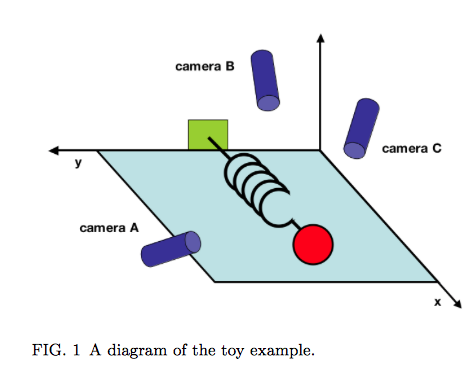
In addition to exploring the assumptions and procedures involved in PCA, Shlens offers a suggestive concrete frame or “toy example” for thinking about it. PCA can be helpful if you want to identify underlying dynamics that have been both captured and obscured by initial measurements of a system. He stages a physical analogy, proposing the made-up situation in which the true axis of movement of a spring must be inferred from haphazardly positioned cameras A, B and C. (That movement is along the X axis.)
Shlens notes that “we often do not know which measurements best reflect the dynamics of our system in question. Furthermore, we sometimes record more dimensions than we actually need!” The idea that the axis of greatest variance is also the axis that captures the “underlying dynamics” of the system is an important one, particularly in a situation where measurements are correlated. This condition is called multicollinearity. We encounter it in text analysis all the time.
If one is willing to entertain the thought that (a) language behaves like a spring across a series of documents and (b) that LATs are like cameras that only imperfectly capture those underlying linguistic “movements,” then PCA makes sense as a tool for dimension reduction. Shlens makes this point very clearly on page 7, where he notes that PCA works where it works because “large variances have important dynamics.” We need to spend more time thinking about what this linkage of variances and dynamics means when we’re talking about features of texts. We also need to think more about what it means to treat individual documents as observations within a larger system whose dynamics they are assumed to express.
Getting to the Projections
How might we go about picturing this mathematical process of orthogonal projection? Shlens’s tutorial focuses on matrix manipulation, which means that it does not help us visualize how the transformation matrix P assists in the projection of the original matrix onto the new bases. But we want to arrive at a more geometrically explicit, and so perhaps intuitive, way of understanding the procedure. So let’s use the code I’ve provided for this post to look at the same data we started with. These are the mean-subtracted values of the Docuscope LATs AbstractConcepts and FirstPerson in the Folger Editions of Shakespare’s plays. To get started, you must place the .csv file containing the data above into your R working directory, a directory you can change using the the Misc. tab. Paste the entire text of the code in the R prompt window and press enter. Within that window, you will now see several means of calculating the covariance matrix (S) from the initial matrix (X) and then deriving eigenvectors (P) and final scores (Y) using both the automated R functions and “longhand” matrix multiplication. If you’re checking, the results here match those derived from the manual operations documented the Excel spreadsheet, albeit with an occasional sign change in P. In the Quartz graphic device (a separate window), we will find five different images corresponding to five different views of this data. You can step through these images by keying control-arrow at the same time.
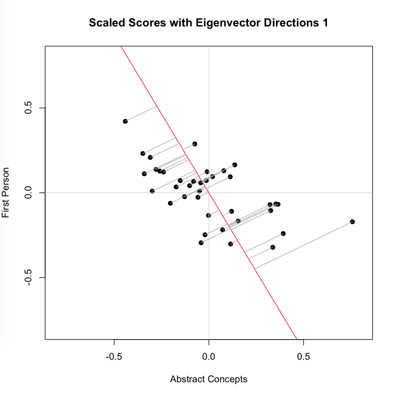
The first view is a centered scatterplot of the measurements above on our received or “naive bases,” which are our two docuscope LATs. These initial axes already give us important information about distances between texts. I repeat the biplot from the top of the post, which shows that according to these bases, Macbeth is the second “closest” play to Henry V (sitting down and to the right of Troilus and Cressida, which is first):
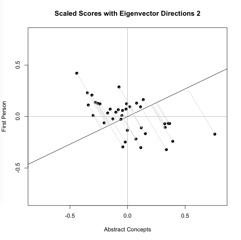
Now we look at the second image, which adds to the plot above a line that is the eigenvector corresponding to the highest eigenvalue for the covariance matrix S. This is the line that, by definition, maximizes the variance in our two dimensional data:You can see that each point is projected orthogonally on to this new line, which will become the new basis or first principal component once the rotation has occurred. This maximum is calculated by summing the squared distances of each the perpendicular intersection point (where gray meets red) from the mean value at the center of the graph. This red line is like the single camera that would “replace,” as it were, the haphazardly placed cameras in Shlens’s toy example. If we agree with the assumptions made by PCA, we infer that this axis represents the main dynamic in the system, a key “angle” from which we can view that dynamic at work.
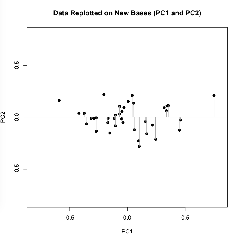
The orthonormal assumption makes it easy to plot the next line (black), which is the eigenvector corresponding to our second, lesser eigenvalue. The measured distances along this axis (where gray meets black) represents scores on the second basis or principal component, which by design eliminates correlation with the first. You might think of the variance along this line is the uncorrelated “leftover” from the that which was captured along the first new axis. As you can see, intersection points cluster more closely around the mean point in the center of this line than they did around the first:
Now we perform the change of basis, multiplying the initial matrix X by the transformation matrix P. This projection (using the gray guide lines above) onto the new axis is a rotation of the original data around the origin. For the sake of explication, I highlight the resulting projection along the first component in red, the axis that (as we remember) accounts for the largest amount of variance:
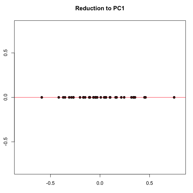
If we now force all of our dots onto the red line along their perpendicular gray pathways, we eliminate the second dimension (Y axis, or PC2), projecting the data onto a single line, which is the new basis represented by the first principal component.
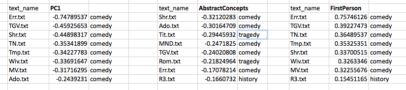
We can now create a list of the plays ranked, in descending order, on this first and most principal component. This list of distances represents the reduction of the two initial dimensions to a single one, a reduction motivated by our desire to capture the most variance in a single direction.
How does this projection change the distances among our items? The comparison below shows the measurements, in rank order, of the far ends of our initial two variables (AbstractConcepts and FirstPerson) and of our new variable (PC1). You can see that the plays have been re-ordered and the distances between them changed:
Our new basis, PC1, looks like it is capturing some dynamic that we might connect to the what the creators of the First Folio (1623) labeled as “comedy.” When we look at similar ranked lists for our initial two variables, we see that individually they too seemed to be connected with “comedy,” in the sense that a relative lack of one (AbstractConcepts) and an abundance of the other (FirstPerson) both seem to contribute to a play’s being labelled a comedy. Recall that these two variables showed a negative covariance in the initial analysis, so this finding is unsurprising.
But what PCA has done is combined these two variables into a new one, which is a linear combination of the scores according to weighted coefficients (found in the first eigenvector). If you are low on this new variable, you are likely to be a comedy. We might want to come up with a name for PC1, which represents the combined, re-weighted power of the first two variables. If we call it the “anti-comedy” axis — you can’t be comic if you have a lot of it! — then we’d be aligning the sorting power of this new projection with what literary critics and theorists call “genre.” Remember that by aligning these two things is not the same as saying one is the cause of the other.
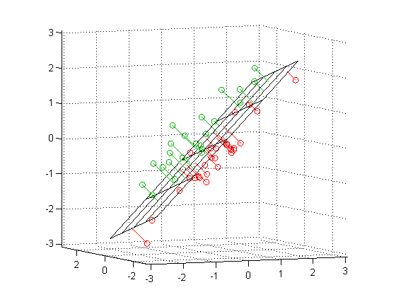
With a sufficient sample size, this procedure for reducing dimensions could be performed on a dozen measurements or variables, transforming that naive set of bases into principal components that (a) maximize the variance in the data and, one hopes, (b) call attention to the dynamics expressed in texts conceived as “system.” If you see PCA performed on three variables rather than two, you should imagine the variance-maximizing-projection above repeated with a plane in the three dimensional space:
Add yet another dimension, and you can still find the “hyperplane” which will maximize the variance along a new basis in that multidimensional space. But you will not be able to imagine it.
Because principal components are mathematical artifacts — no one begins by measuring an imaginary combination of variables — they must be interpreted. In this admittedly contrived example from Shakespeare, the imaginary projection of our existing data onto the first principal component, PC1, happens to connect meaningfully with one of the sources of variation we already look for in cultural systems: genre. A corpus of many more plays, covering a longer period of time and more authors, could become the basis for still more projections that would call attention to other dynamics we want to study, for example, authorship, period style, social coterie or inter-company theatrical rivalry.
I end by emphasizing the interpretability of principal components because we humanists may be tempted to see them as something other than mathematical artifacts, which is to say, something other than principled creations of the imagination. Given the data and the goal of maximizing variance through projection, many people could come up with the same results that I have produced here. But there will always be a question about what to call the “underlying dynamic” a given principal component is supposed to capture, or even about whether a component corresponds to something meaningful in the data. The ongoing work of interpretation, beginning with the task of naming what a principal component is capturing, is not going to disappear just because we have learned to work with mathematical — as opposed to literary critical — tools and terms.
Axes, Critical Terms, and Motivated Fictions
Let us return to the idea that a mathematical change of basis might call our attention to an underlying dynamic in a “system” of texts. If, per Shlens’s analogy, PCA works by finding the ideal angle from which to view the oscillations of the spring, it does so by finding a better proxy for the underlying phenomenon. PCA doesn’t give you the spring, it gives you a better angle from which to view the spring. There is nothing about the spring analogy or about PCA that contradicts the possibility that the system being analyzed could be much more complicated — could contain many more dynamics. Indeed, there nothing to stop a dimension reduction technique like PCA from finding dynamics that we will never be able to observe or name.
Part of what the humanities do is cultivate empathy and a lively situational imagination, encouraging us to ask, “What would it be like to be this kind of person in this kind of situation?” That’s often how we find our way into plays, how we discover “where the system’s energy is.” But the humanities is also a field of inquiry. The enterprise advances every time someone refines one of our explanatory concepts and critical terms, terms such as “genre,” “period,” “style,” “reception,” or “mode of production.”
We might think of these critical terms as the humanities equivalent ofamathematical basis on which multidimensional data are projected. Saying that Shakespeare wrote “tragedies” reorients the data and projects a host of small observations on a new “axis,” as it were, an axis that somehow summarizes and so clarifies a much more complex set of comparisons and variances than we could ever state economically. Like geometric axes, critical terms such as “tragedy” bind observations and offer new ways of assessing similarity and difference. They also force us to leave things behind.
The analogy between a mathematical change of basis and the application of critical terms might even help explain what we do to our colleagues in the natural and data sciences. Like someone using a transformation matrix to re-project data, the humanist introduces powerful critical terms in order to shift observation, drawing some of the things we study closer together while pushing others further apart. Such a transformation or change of basis can be accomplished in natural language with the aid of field-structuring analogies or critical examples. Think of the perspective opened up by Clifford Geertz’s notion of “deep play,” or his example of the Balinese cock fight, for example. We are also adept at making comparisons that turn examples into the bases of new critical taxonomies. Consider how the following sentence reorients a humanist problem space: “Hamlet refines certain tragic elements in The Spanish Tragedy and thus becomes a representative example of the genre.”
For centuries, humanists have done these things without the aid of linear algebra, even if matrix multiplication and orthogonal projection now produce parallel results. In each case, the researcher seeks to replace what Shlens calls a “naive basis” with a motivated one, a projection that maps distances in a new and powerful way.
Consider, as a final case study in projection, the famous speech of Shakespeare’s Jacques, who begins his Seven Ages of Man speech with the following orienting move: “All the world’s a stage, / And all the men and women merely players.” With this analogy, Jacques calls attention to a key dynamic of the social system that makes Shakespeare’s profession possible — the fact of pervasive play. Once he has provided that frame, the ordered list of life roles falls neatly into place.
This ability to frame an analogy or find an orienting concept —the world is a stage, comedy is a pastoral retreat, tragedy is a fall from a great height, nature is a book — is something fundamental to humanities thinking, yet it is necessary for all kinds of inquiry. Improvising on a theme from Giambattista Vico, the intellectual historian Hans Blumenberg made this point in his work on foundational analogies that inspire conceptual systems, for example the Stoic theater of the universe or the serene Lucretian spectator looking out on a disaster at sea. In a number of powerful studies — Shipwreck with Spectator, Paradigms for a Metaphorology, Care Crosses the River — Blumenberg shows how analogies such as these come to define entire intellectual systems; they even open those systems to sudden reorientation.
We certainly need to think more about why mathematics might allow us to appreciate unseen dynamics in social systems, and how critical terms in the humanities allow us to communicate more deliberately about our experiences. How startling that two very different kinds of fiction — a formal conceit of calculation and the enabling, partial slant of analogy — help us find our way among the things we study. Perhaps this should not be surprising. As artifacts, texts and other cultural forms are staggeringly complex.
I am confident that humanists will continue to seek alternative views on the complexity of what we study. I am equally confident that our encounters with that complexity will remain partial. By nature, analogies and computational artifacts obscure some things in order to reveal other things: the motivation of each is expressed in such tradeoffs. And if there is no unmotivated view on the data, the true dynamics of the cultural systems we study will always withdraw, somewhat, from the lamplight of our descriptive fictions.
Let’s say that we believe we can learn something more about what literary critics call “authorial style” or “genre” by quantitative work. We want to say what that “more” is. We assemble a community of experts, convening a panel of early modernists to identify 10 plays that they feel are comedies based on prevailing definitions (they end in marriage), and 10 they feel are tragedies (a high born hero falls hard). To test these classifications, we randomly ask others in the profession (who were not on the panel) to sort these 20 plays into comedies and tragedies and see how far they diverge from the classifications of our initial panel. That subsequent sorting matches the first one, so we start to treat these labels (comedy/tragedy) as “ground truths” generated by “domain experts.” Now assume that I take a computer program, it doesn’t matter what that program is, and ask for it to count things in these plays and come up with a “recipe” for each genre as identified by our experts. The computer is able to do so, and the recipes make sense to us. (Trivially: comedies are filled with words about love, for example, while tragedies use more words that indicate pain or suffering.) A further twist: because we have an unlimited, thought-experiment budget, we decide to put dozens of early modernists into MRI machines and measure the activity in their brains while they are reading any of these 20 plays. After studying the brain activity of these machine-bound early modernists, we realize that there is a distinctive pattern of brain activity that corresponds with what our domain experts have called “comedies” and “tragedies.” When someone reads a comedy, regions A, B and C become active, whereas when a person reads tragedies, regions C, D, E, and F become active. These patterns are reliably different and track exactly the generic differences between plays that our subjects are reading in the MRI machine.
So now we have three different ways of identifying – or rather, describing – our genre. The first is by expert report: I ask someone to read a play and she says, “This is a comedy.” If asked why, she can give a range of answers, perhaps connected to plot, perhaps to her feelings while reading the play, or even to a memory: “I learned to call this and other plays like it ‘comedies’ in graduate school.” The second is a description, not necessarily competing, in terms of linguistic patterns: “This play and others like it use the conjunction ‘if’ and ‘but’ comparatively more frequently than others in the pool, while using ‘and’ less frequently.” The last description is biological: “This play and others like it produce brain activity in the following regions and not in others.” In our perfect thought experiment, we now have three ways of “getting at genre.” They seem to be parallel descriptions, and if they are functionally equivalent, any one of them might just be treated as a “picture” of the other two. What is a brain scan of an early modernist reading comedy? It is a picture of the speech act: “The play I’m reading right now is a comedy.”
Now the question. The first three acts of a heretofore unknown early modern play are discovered in a Folger manuscript, and we want to say what kind of play it is. We have our choice of either:
• asking an early modernist to read it and make his or her declaration
• running a computer program over it and rating it on our comedy/tragedy classifiers
• having an early modernist read it in an MRI machine and characterizing the play on the basis of brain activity.
Let’s say, for the sake of argument, that you can only pick one of these approaches. Which one would you pick, and why? If this is a good thought experiment, the “why” part should be challenging.
Several years ago I did some experiments with Franco Moretti, Matt Jockers, Sarah Allison and Ryan Heuser on a set of Victorian novels, experiments that developed into the first pamphlet issued by the Stanford Literary Lab. Having never tried Docuscope on anything but Shakespeare, I was curious to see how the program would perform on other texts. Looking back on that work, which began with a comparison of tagging techniques using Shakespeare’s plays, I think the group’s most important finding was that different tagging schemes can produce convergent results. By counting different things in the texts – strings that Docuscope tags and, alternatively, words that occur with high frequency (most frequent words) – we were able to arrive at similar groupings of texts using different methods. The fact that literary genres could be rendered according to multiple tagging schemes sparked the idea that genre was not a random projection of whatever we had decided to count. What we began to think as we compared methods, and it is as exciting a thought now as it was then, was that genre was something real.
Real as an iceberg, perhaps, genre may have underwater contours that are invisible but mappable with complementary techniques. Without delving too deeply into the specifics of the pamphlet, I’d like to sketch its findings and then discuss them in some of the terms I outlined in the previous post on critical gestures. First the preliminaries. In the initial experiment, we established a corpus (the Globe Shakespeare) and then used two tagging schemes to assign the tokens into those documents to a smaller number of types. (This is the crucial step of reducing the dimensionality of the documents, or “caricaturing” them.) The first tagging scheme, Docuscope, rendered the plays as percentage scores on the types it counts; the second, implemented by Jockers, identified the most frequent words (MFWs) in the corpus and likewise used these as the types or variables for analysis.
What we found was that the circles drawn by critics around these texts – circles here bounding different genres – could be reproduced by multiple means. Docuscope’s hand-curated tagging scheme did a fairly good job of reproducing the genre groupings via an unsupervised clustering algorithm, but so did the MFWs. We were excited by these results, but also cautious. Perhaps the words counted by Docuscope might include the very MFWs that were producing such good results in the parallel trial, which would mean we were working with one tokenization scheme rather than two. Subsequent experiments on Victorian novels curated by the Stanford team – for example, a comparison of the Gothic Novel versus Jacobin (see pp. 20-23) – showed that Docuscope was adding something over and above what was offered by counting MFWs. MFWs such as “was,” “had,” “who,” and “she,” for example were quite good at pulling these two groups apart when used as variables in an unsupervised analysis. But these high frequency words, even when they composed some of the Docuscope types that were helpful in sorting the genres, were correlated with other text strings that were more narrative in character, phrases such as “heard the,” “reached the,” and “commanded the.” So while we had some overlap in the two tagging schemes, what they shared did not explain the complementary sorting power each seemed to bring to the analysis. The rhetorical and semantic layers picked out in Docuscope were, so to speak, doing something alongside the more syntactically important function words that occur in texts with such high frequency.
The nature of that parallelism or convergence continues to be an interesting subject for thought as we discover more tagging schemes and contemplate making our own. Discussions in the NEH sponsored Early Modern Digital Agendas workshop at the Folger, some of which I have been lucky enough to attend, have pushed Hope and me to return to the issue of convergence and think about it again, especially as we think about how our research project, Visualizing English Print, 1470-1800, might implement new tagging schemes. If MFWs produce viable syntactical criteria for sorting texts, why would this “layer” of syntax be reliably coordinated with another, Docuscope-visible layer that is more obviously semantic or rhetorical? If different tagging schemes can produce convergent results, is it because they are invoking two perspectives on a single entity?
Because one doesn’t get completely different groupings of texts each time one counts new things, we must posit the existence of something underneath all the variation, something that can be differently “sounded” by counting different things. The main attribute of this entity is its capacity to encourage or limit certain sorts of linguistic entailments. As I think back on how the argument developed in the Stanford paper with Moretti et al., the crucial moment came when we found that we could describe the Gothic novel as having both more spatial prepositions (“from,” “on,” “in,” “to”) and more narrative verb phrases (“heard the,” “reached the”) than the Jacobin novel. Our next move was to begin asking whether either of the tagging schemes was picking out a more foundational or structural layer of the text – whether, for example, the decision to use a certain type of narrative convention and, so, narrative phrase, entailed the use of corresponding spatial prepositions. As soon as the word “structural” appeared, I think everyone’s heart began to beat a little faster. But why? What is so special about the word “structural,” and what does it mean?
In the context of this experiment, I think “structural” means “is the source of the entailment;” its use, moreover, suggests that the entailment has direction. We (the authors of the Stanford paper) were claiming that, in deciding to honor the plot conventions of a particular generic type, the writer of a Gothic novel had already committed him or herself to using certain types of very frequent words that critics tend to ignore. The structure or plot was obligating, perhaps in an unconscious way.
I think now that I would pause before using the word “structure,” a word used liberally in that paper, not because I don’t think there is such a thing, but because I don’t know if it is one or many things. Jonathan Hope and I have been looking for a term to describe the entailments that are the focus of our digital work. We have chose to adopt, in this context, a deliberately “fuzzy structuralism” when talking about entailments among features in texts. We would prefer to say, that is, that the presence of one type of token (spatial preposition) seems to entail the presence of another type (narrative verb phrases), and remain agnostic about the direction of the entailment. Statistical analysis provides evidence of that relationship, and it is the first order of iterative criticism to describe such entailments, both exhaustively (by laying bare the corpus, counts, and classifying techniques) and descriptively (by identifying, through statistical means, passages that exemplify the variables that classify the texts most powerfully). Just as important, we feel one ought where possible to assign a shorthand name – “Gothicness,” “Shakespearean” – to the features that help sort certain kinds of texts. In doing so, we begin to build a bridge connecting our linguistic description to certain already known genre conventions that critics recognize or “circle” in their own thinking. But the application of the term”Gothic,” and the further claim that this names the cause of the entailments we discern by multiple means, deserves careful scrutiny.
A series of questions about this entailment entity, then, which sits just under the waterline of our immediate reading:
• How does entailment work? This is a very important question, since it gets at the problem of layers and depth. At one point in the work with the Stanford team, Ryan Heuser offered the powerful analogy alluded to above: genre is like an iceberg, with features visible above the water but depths unseen below. Plot, we all agreed, is an above the waterline phenomenon, whereas MFW word use and certain semantic choices are submerged below the threshold of conscious attention. In the article we say that the below-the-waterline phenomena sounded by our tagging schemes are entailed by the “higher order” choices made when the writer decided to write a “Gothic novel” or “history play.” I still like this idea, but worry it might suggest that all features of genre are the result of some governing, genre-conscious choice. What if some writers, in learning to mimic other writers, take sentence level cues and work “upward” from there? Couldn’t there be some kind of semi-conscious or sentence-based absorption of literary conventions that is specifically not a mimicry of plot?
• Are the entailments pyramidal, with a governing apex at the top, or are they multi-nodal and so radiating from different points within the entity? I can see how syntax, which is mediated by function or high-frequency words, is closely tied to certain higher order choices. If I want to write stories about lovers who don’t get along, this will entail using a lot of singular pronouns in the first and second person alongside words that support mutual misunderstanding. There is a relationship of entailment between these two things, and the source of that entailment is often called “plot” or “genre.” Here again we are at an interpretive turning point, since the names applied to types of texts are as fluid, at least potentially, as those assigned to types of words. Such names can be misleading. Suppose, for example, that I have identified the distinct signature of something like a “Shakespearean sentence,” and that this signature is apparent in all of Shakespeare’s plays. (An author-specific linguistic feature set was created for J. K. Rowling just last week.) Suppose further that, as Shakespeare is almost singlehandedly launching the history play as a theatrical genre in the 1590s, this authorial feature propagates alongside the plot-level features he establishes for the genre. Now someone shows that this Shakespearean sentence signature is reliably present in most plays that critics now call histories. Is that entailment upheld by the force of genre or authorship? The question would be just as hard to answer if we noticed that the generic signal of history plays spans the rest of Shakespeare’s writing and is a useful feature for differentiating his works from those of other authors.
• If entailments can be resolved at varying depths of field, like the two cats below, which are simultaneously resolved by the Lytro Camera at multiple focal lengths, how can we be sure that they are individual pieces of a single entity or scene? Different tagging schemes support the same groupings of texts, so there must be something specific “there” to be tagged which has definite contours. I remain astonished that the groupings derived from tagging schemes like Docuscope and MFWs correspond to names we use in literary criticism, names that designate authors and genres of fiction. But entailments are plural: some seem to correspond to what we call authorship, others genre, and perhaps still others to the medium itself (the small twelvemo, for example, often contains different kinds of words than those found in the larger folio format). There are biological constraints on how long we can attend to a single sentence. The nature and source of these entailments has thus got to be the subject of ongoing study, one that bridges a range of fields as wide as there are forces that constrain language use.
Entailment is real; it suggests an entity. But how should we describe that entity, and with what terms or analogies can its depths be resolved? Sometimes there may be multiple cats, sitting apart in the same room. Sometimes what seems like two icebergs may in fact be one.
Image from the Lytro Camera resolving objects at multiple depths


 Plotting the items in two dimensions gives the viewer some general sense of the shape of the data. “There are more items here, less there.” But when it comes to thinking about distances between texts, we often measure straight across, favoring either a simple line linking two items or a line that links the perceived centers of groups.
 To get started, you must place the
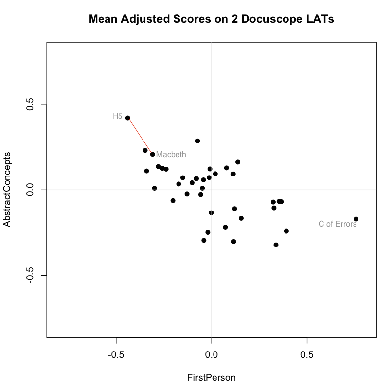
 You can see that each point is projected orthogonally on to this new line, which will become the new basis or first principal component once the rotation has occurred. This maximum is calculated by summing the squared distances of each the perpendicular intersection point (where gray meets red) from the mean value at the center of the graph. This red line is like the single camera that would “replace,” as it were, the haphazardly placed cameras in Shlens’s toy example. If we agree with the assumptions made by PCA, we infer that this axis represents the main dynamic in the system, a key “angle” from which we can view that dynamic at work.